YSOVAR Data Description Document

Table of Contents:

• I. Overview of the YSOVAR Orion Observing Program
• II. Pipeline processing
• III. The Sample of Stars with Delivered Photometry
• IV. Data Products Provided Here
• V. The YSOVAR Orion Database Interface
• VI. Caveats and Cautions for the ONC Photometry

I. Overview of the YSOVAR Orion Observing Program

YSOVAR is a Spitzer Cycle 6 Exploration Science Program (PI: J. Stauffer). Cycle 6 was the first call for proposals for observations to be obtained after Spitzer's cryogen was exhausted. The Exploration Science programs were defined as large programs in excess of 500 hours of requested observing time. YSOVAR was approved for 550 hours of time, with the goal of obtaining the first extensive mid-infrared time-series photometry of the central part of the Orion Nebula Cluster plus eleven other, smaller star-forming cores. YSOVAR data should help reveal the structure of the inner disk region of YSOs, provide new constraints on accretion and extinction variability, identify new PMS eclipsing binaries, and help identify new very low mass substellar members of the surveyed clusters.

Almost half of the allocated YSOVAR Spitzer observing time was devoted to time series photometry of a 0.9 square degree region centered on the Trapezium cluster in Orion, beginning on October 24, 2009 and lasting for 40 days (essentially the entire Spitzer visibility window for Orion). On average, two epochs of observation were obtained on each day, but the interval between observations was varied both by design (to minimize period-aliasing problems) and due to constraints imposed by other Spitzer programs that were executed during the same campaigns. The FOV at one epoch is shown in Figure 1 below. The exact region covered at each epoch varied slightly because the orientation of the IRAC detector on the sky varies with time. The inner part of the ONC was observed with a short (1.2s) integration time and 20 small dithers in order to keep the sky background rate below saturation. The outer part of the ONC was observed in high-dynamic range mode, with 10.4 and 0.4 sec integration times and 4 dithers. The outline of the approximate region observed with the short integration times is shown in Figure 1.

In addition to the IRAC data, we also obtained optical and near-IR time series photometry for the same region during October through December 2009. These data were obtained with a variety of telescopes (SLOTIS, APO, CFHT, UKIRT, as well as others). The details of each telescope/camera and set of observations is provided in Table 1. For this first release of the processed data from the Orion YSOVAR observations, we only provide data from the four facilities explicitly mentioned above.

First results on this project can be found in Morales-Calerón, M. et al. 2011, ApJ

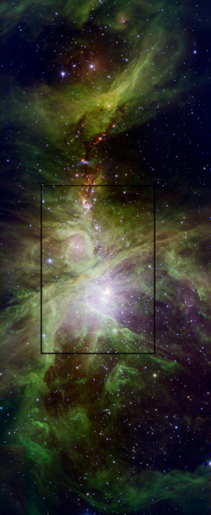
Figure 1: Color image of the observed area. The black square in the center denotes the approximate location of the inner part of the observations, taken with shorter exposure times to limit saturation.

Table 1: Ancillary Supporting Observation Details

Telescope	Instrument	Filter	Start/End dates	N Epochs	Central Coordinates (J2000)	Area (arcmin)	Exptime/Epoch (sec.)
UKIRT	WFCAM	J	Oct. 20 - Dec. 22, 2009	32	5:35:17 -05:22:49	52x104	2x3
CFHT	WIRCam	J,Ks	Oct. 27 - Nov. 8, 2009	11	05:35:14 -04:41:34	21x21	(5x2)x7(J), 5x7(Ks)
					05:35:14 -05:02:14
					05:36:04 -05:22:46
					05:34:26 -05:22:46
					05:35:14 -05:43:28
NMSU APO1m	CCD	Ic	Oct. 24, 2009 - Feb. 09, 2010	27	05:35:18 -05:24:03	15x15	60x20
SuperLotis	CCD	Ic	Oct. 28 - Dec. 12, 2009	23	05:35:11 -05:41:02	16x16	180x12

II. Pipeline processing

The currently available Orion photometry derives from BCDs processed at the Spitzer Science Center in late 2009 using the S18.12 software build. For each epoch, the BCDs were fed through the IDL package Cluster Grinder (Gutermuth et al. 2009). Each BCD was processed for standard bright source artifacts and combined into mosaics (at 0.86" per pixel grid resolution) by epoch and bandpass. Then point sources were automatically detected and aperture photometry obtained from these mosaics. The aperture radius used was 2.4 arcseconds, with a sky annulus having inner and outer radii of 2.4 and 7.2 arcseconds; to calibrate these measurements, we adopted Vega standard magnitude zero points of 19.30 and 18.67 for 1 DN/s total flux at 3.6 and 4.5 microns, respectively. These values include standard corrections for our chosen aperture and sky annulus sizes (Reach et al. 2005). Uncertainties were derived by combining three terms in quadrature: shot noise in the aperture, shot noise in the mean background flux per pixel integrated over the aperture, and the standard deviation of the sky annulus pixels (to account for the influence of non-uniform nebulous background).

For the ground-based photometry, in each case, the raw images were processed either by the observer or by a home institute which maintains a dedicated pipeline, yielding flat-fielded, bias subtracted images to which a reasonably accurate WCS has been attached. The ground-based data were obtained at a sparser cadence than the Spitzer observations, and in some cases includes epochs from outside the Spitzer visibility window (see Table 1). Aperture photometry was performed on each epoch of data using aperture sizes of 1 to 3 arcsec, depending on the PSF and pixel scale of the camera. In each dataset, for each object, an artificial reference level was created by selecting a set of median filtered nearby, non-variable comparison stars. For the UKIRT data, the images and catalogs for each individual epoch delivered by the WFCAM science archive are fully calibrated. For the other datasets, the photometry was put on an absolute scale by determining the mean difference between a calibrated dataset (2MASS or the I-band data from Hillenbrand, L. A. 1997, AJ, 113, 1733) and our new photometry. The errors listed in the database correspond to the values produced by the photometry package.

III. The Sample of Stars with Delivered Photometry

Even though the ONC is a rich young cluster, and even though the Orion molecular cloud acts to greatly limit the number of background objects detected towards the ONC, known Orion members comprise only a very small fraction of the objects detected in our images. In this delivery, we provide time series photometry only for stars identified as probable ONC members. We split the member list into two samples. The first set of about 1400 objects are stars falling in the region we surveyed that were identified as having IR excesses using data from the Spitzer GTO survey of Orion obtained during the cryogenic mission (Megeath et al. 2011). These objects are by definition almost all either Class I or Class II YSOs. The second set of over 1000 objects are stars in our survey region that are identified in the literature as being ONC members, but which are not included in the IR-excess sample. The great majority of these objects are Class III YSOs (WTTs), but a few may be Class IIs whose IR excesses were not convincing enough to include in the Megeath et al. sample. The second set of stars is primarily composed of X-ray sources and proper-motion-selected candidate members. While we have done our best, it is likely that a few of the stars in both catalogs are actually not members of the ONC; it is also likely true that another set of ONC members remain unidentified in our survey region, yet have acceptable light curves. Note also that in this release we exclude some stars where we have very incomplete IRAC data or where the IRAC data are problematic for some reason; we will attempt to include the data for some of these stars in a future release.

Naming Convention: Stars are named following the IAU convention using an acronym (Initial Spitzer Orion Ysovar: ISOY) followed by the J2000 coordinates.

IV. Data Products Provided in this Delivery

Imaging: data from the YSOVAR survey and from the 2MASS Orion variability survey:

• A JPEG color image of the FOV we surveyed (about 25' x 90'), combining K band data from 2MASS (blue), 3.6 micron (green) and 4.5 micron (red).

• A JPEG color image of the FOV we surveyed (about 25' x 90'), combining 3.6 micron (blue) and 4.5 micron (brown).

• FITS files for the 3.6 and 4.5 micron mosaics built by combining all the data retrieved during the first two weeks of observation, covering the region shown in Figure 1.

Photometry: Two files provide basic information for ONC members for which we provide light curves:

• Table: ONC Stars with IR Excesses - This file provides the name, aliases, RA, Dec, J,H,K, [3.6], [4.5], [5.8] and [8.0] magnitudes for the 1396 candidate ONC members as identified by Megeath et al. (2011) in our FOV (Notes: tabulated uncertainties are the relative photometric uncertainties determined by the photometry software the calibration uncertainty should be < 5%).

• Table: ONC candidate members not known to have IR Excesses - This file provides the name, aliases, RA, Dec, J,H,K, [3.6], [4.5], [5.8] and [8.0] magnitudes for the 1027 ONC members in our FOV not identified as having IR excesses in Megeath et al. (2011) Notes: tabulated uncertainties are the relative photometric uncertainties determined by the photometry software the calibration uncertainty should be < 5%).

• Two files provide plots of multi-wavelength light curves for the Oct. 24 - Dec. 4 time period for the Orion members in our FOV. The y-axis for these plots is generally the [4.5] magnitude; for other bands, a zero-point shift has been added to the photometry to align it with the 4.5 micron data but the same delta-magnitude range is used for all bands - i.e. if the total range in [4.5] is 0.4 mag, that is also the same range shown for the other bands.
  • Plot: Light Curves for IR excess members [Table 1 above].

  • Plot: Light Curves for WTTS, e.g., likely members without infrared excess [Table 2 above].

• Finally, tar files are provided which include all of the Orion time series photometry in a set of ascii tables:
  • IRAC1 gzipped tar file
  • IRAC2 gzipped tar file
  • J UKIRT gzipped tar file
  • J CFHT gzipped tar file
  • K CFHT gzipped tar file
  • I APO gzipped tar file
  • I SLOTIS gzipped tar file

V. The YSOVAR Orion Database Interface

An alternative means to view and access the YSOVAR Orion data is through a database interface. The interface allows a user to run SQL queries to select stars with a given set of properties, or to see the data for a particular star. The user can either simply view the light curve or download the data. A few of the most commonly-used examples of SQL queries are given below.

The YSOVAR main query page

This main menu allows to search the YSOVAR database using either the empty fields or sql queries as follows: (note however that a mixed search using both fields and sql queries at the same time won't work)

Target Name: stars are named following the IAU convention using an acronym (Initial Spitzer Orion Ysovar: ISOY) followed by the J2000 coordinates - e.g. ISOY_J053508.53-052518.0. An object can also be searched by its Alias Name. Note that the database is case sensitive.

Cone search: sources can be searched by coordinates using the database cone search both with decimal degrees or sexagesimal positions. Acceptable formats are:

• RAdeg +-DEdeg radius(in arcsec) (at this time only this option is available!)
• HH:MM:SS +-DD:MM:SS radius (in arcsec)

Telescope: this is a pulldown menu which allows to specify the source of the data. The data available in the database come from Spitzer, UKIRT, CFHT, NMSU-APO 1m, and Super Lotis telescopes.

Useful Pre-defined Queries: here you can find several useful pre-defined sql queries. See below for more useful queries or if you would like to design your own.

Your Own SQL query: here you can define your own sql query. See below for several examples of customized queries. Notes on queries:

• Naming convention and format for the quantities available through the database can be found in the DB schema. Short descriptions for those quantities available can be found in the DB descriptions.
• to be able to sort and navigate through pages of the query result, the first column of your query result has to contain unique entries (e.g., running numbers or IDs). Otherwise, you will see only the 1st page of the query result.
• the "order by" command is handled by the database and thus cannot be used by the user. Queries will return results in the order as they are stored in the database.
• the database is case sensitive (the 'case' command can be used to override that).

Seeing and Downloading data

Once you have done your query you will be able to see the results as a table on the screen you can also download the data by clicking on "download data".

The file that is created will be a gzipped, ".csv" file (comma separated value). If you use Firefox, it will recognize the file is in fname.csv.gz format. If you use Safari, unfortunately, it does not recognize it is a gzipped file, and just names it "fname.csv". You will need to rename the file (add a ".gz" suffix), then run gunzip manually.

Note: Mag = -100: non-detection; Unc = -100: non-detection or questionable detection;

Browsing and filtering the database

Instead of making a query you can browse and filter the database by clicking on the "Browse" button on the top left corner.

Doing that will give you a list of all the sources in the database, with some default columns: Name: Target Name, Alias: Alias Name, RA and DEC: averaged sexagesimal coordinates, Member, N: number of useful datapoints in the light curves, Avg_Mag: mean magnitude computed whithin the database, Sigma_mag: standard deviation in the light curve computed whithin the database, Filter, Telescope, cluster, source id, and link. The last column, link, gives you a link to the light curve (LC) of that source. If you click on a point of the light curve, then you will see specific information on that data point, including a postage-stamp cutout from the image from which that photometry value was derived. Note that any column whithin the browser can be sorted.

To filter the database you can click on the magnifying button at the bottom left corner and you'll get a set of buttons you can use to set specific values or ranges for the filtering. The following columns can be filtered: Name: stars are named following the IAU convention using an acronym (Initial Spitzer Orion Ysovar: ISOY) followed by the J2000 coordinates - e.g. ISOY_J053508.53-052518.0. Note that the database is case sensitive.

Alias: this is an internal name which looks like: ORION-ClassI-*, ORION-ClassII-*, ORION-Mem-*, or ORION-* depending on if they are ClassI, ClassII, objects that have been specifically claimed to be members (based on proper motion or spectroscopic studies) with no IR excess detected, or members of the cluster selected from some reason different from proper motion (such as variability or spectroscopic signatures) with no IR excess detected. These names are generally not known by the public. However, if you know the number of a star (say ORION-ClassII-790) you can search it using %-790 in the Alias Name field or even you can search for objects with IR excess by typing %Class% in the Alias Name field. Note that in the main query page, in the Target Name field you can use either target name or alias name. In the browse menu however, there are two different fields for Target Name and Alias Name. The database is case sensitive.

rahms and dedms: sexagesimal coordinates averaged over the whole observing period.

Member: a value of 2 is asigned to members however note that only Orion members are being released in this initial release.

Filter: pulldown menu with the available bands: I, J, K, IRAC1, and IRAC2.

Telescope: this is a pulldown menu which allows to specify the source of the data. The data available in the database come from Spitzer, UKIRT, CFHT, NMSU-APO 1m, and Super Lotis telescopes.

Cluster: all the data available in the database are from Orion.

Source ID: running number that is automatically assigned to a source when first ingested in the database. Note that this number will change if there is a need of repopulating the database. It is strongly advised to keep note of the Target Name or coordinates of any source you want to keep track on.

N: these fields allow to search for objects with a specific number of useful measurements. Note that the number under 'From' must be lower than that under 'To'.

Avg_mag: these fields allow to search for objects in a specific range of average magnitudes. Note that the number under 'From' must be lower than that under 'To'.

Sigma_mag: these fields allow to search for objects with a standard deviation from the mean magnitude in a specific range determined by the values 'From' and 'To'. Note that the number under 'From' must be lower than that under 'To'.

Note that if you download the data after filtering you will still be getting all the Orion data, not just the filtered dataset.

Plotting the Light Curves

If you know the name of the star in the database, you can type that name into the "Target Name" box on the front page.

If you do not know the name of the star in the database, but you do know its exact coordinates (hh:mm:ss.ss, dd:mm:ss.s), you can type in the coordinates as described above.

If you just know the approximate coordinates, you can use the "Browse" tab to display all the members of Orion, and then click on the top of the RA column - the stars will then be sorted by Right Ascension, and you can scan down through the list until you come to your star.

Once you have the source you want, you just have to click on the link on the right (LC) to see the light curve . If you click on a point of the light curve, then you will see specific information on that data point, including a postage-stamp cutout from the image from which that photometry value was derived.

Custom queries

Here there are a few examples of sql queries that can be useful:

a) How to Download Light Curves for a Specific Star

To get all the data for one star you need to use an SQL query.

select s.name as sname,mjd, f.name as fname, mag1, emag1 from source s,photom p,filter f where s.id=p.source_id and s.name='ISOY_J053413.20-053353.6' AND f.id=p.filter

Another page should show up, with one row for each filter and epoch - for that star.

Click on "download data".

The file that is created will be a gzipped, ".csv" file (comma separated value). If you use Firefox, it will recognize the file is in fname.csv.gz format, and will unzip it for you. If you use Safari, unfortunately, it does not recognize it is a gzipped file, and just names it "fname.csv". You will need to rename the file (add a ".gz" suffix), then run gunzip manually.

Note that the resultant file is not time-ordered. It also has data for the different filters, in no particular order. You will need to sort the data as you desire before using it.

b) How to Retrieve a Light Curve At a Single Band for a specific star:

select s.name as sname,mjd,mag1,emag1,f.name from source s, photom p,filter f where s.id=p.source_id and s.name='ISOY_J053413.20-053353.6' and f.id=p.filter and f.name='IRAC2'

Where IRAC2 is the band you want. Other bands available are I, J, K, and IRAC1. Note that the resultant file is not time-ordered.

c) How to Retrieve a Light Curve At a Single Band for all Objects in Orion:

select s.name as sname,mjd, f.name as fname, mag1, emag1 from source s,photom p,filter f where s.id=p.source_id and f.id=p.filter and f.name='IRAC1' and cluster=10

Where IRAC1 is the band you want. Other bands available are I, J, K, and IRAC2. Note that the resultant file is not time-ordered, however the sources are: you'll get all the data for object 1 then object 2 and so on.

d) How to Retrieve Light Curves At all Bands for all Objects in Orion:

select source.name as sname,mjd,mag1,emag1,filter.name as fname from photom,source,filter where photom.source_id=source.id and cluster=10 and photom.filter=filter.id

Note that in this case, even when the different bands are not ordered, the sources are. You'll get all the data for object 1 then object 2 and so on. Note that the sql queries cannot be used at the same time as the web queries.

e) How to download the light curves for a specific YSO class:

To get all the sources classified as ClassI in the band IRAC1:

SELECT s.name as sname,p.mjd,f.name as fname, p.mag1,p.emag1 FROM source s, photom p, filter f, alias a WHERE s.id = p.source_id AND p.filter = f.id AND s.id = a.id AND f.name = 'IRAC1' AND a.name like '%ClassI-%' AND cluster = 10 To get all the sources classified as ClassII in the band IRAC2:

SELECT s.name as sname,p.mjd,f.name as fname, p.mag1,p.emag1 FROM source s, photom p, filter f, alias a WHERE s.id = p.source_id AND p.filter = f.id AND s.id = a.id AND f.name = 'IRAC2' AND a.name like '%ClassII%' AND cluster = 10 To get all the sources with no IR excess in the I band:

SELECT s.name as sname,p.mjd,f.name as fname, p.mag1,p.emag1 FROM source s, photom p, filter f, alias a WHERE s.id = p.source_id AND p.filter = f.id AND s.id = a.id AND f.name = 'I' AND a.name not like '%ClassI%' AND cluster = 10 and useful = 1

f) How to cluster and count different populations:

SELECT c.name, count(class1), count(class2), count(class3), count(*) FROM (SELECT s.id, cluster, case when a.name like '%classI-%' then TRUE else null end as class1, case when a.name like '%classII%' then TRUE else null end as class2, case when a.name not like '%classI%' then TRUE else null end as class3 FROM source s inner join alias a on (s.id = a.id)) sa inner join cluster c on (sa.cluster = c.id) GROUP BY c.id

The trick is to create a column for each class that is non-null if and only if the star is a member of that class. One can then add up the number of stars in each class just by using count, which ignores nulls

VI. Caveats and Cautions for the ONC Photometry

IRAC data:

• FOV rotates with time - we do not have data for some stars at some intervals (examples are: objects J053429.56-044502.6 and J053600.86-044258.7)

• When a star comes into the FOV, the photometry is sometimes bad for several days due to edge effects. We provide this photometry, but flag the suspect values in the database and on the plots shown by the database interface. Note that the data is only flagged in the database, the ascii files we provide contain all the epochs with no flags

• There are edges of the FOV where we only have 3.6 or 4.5, not both (examples are objects J053548.14-055357.3 and J053550.49-055142.3)

• There are regions where we have HDR (12, 0.6 sec) data and other regions with 2 sec data. This is a result of trying to deal with nebular background (see Figure 1).

• HDR mode means that in some cases we have 2 measures of the star's flux at each epoch. But these may have slightly different zero point offsets or one of the sets may be noisy/saturated. This can cause there to be more than 80 IRAC points in the light curves or for there to be two data points at a given epoch for one or both channels. (examples are: J053524.24-052957.3 and J053505.62-052922.3)

• Diffraction spikes of bright stars rotate with time - if a target star falls near a diffraction spike, this can introduce false variability. (examples are: the fainter stars near 2MASS J05354506-0517496)

• Structured nebulosity yields added noise and a variable faint magnitude limit.

• Other artifacts (latent images, bad pixels, asteroids) can cause either single photometry points or all the data for intervals of a few days to a week or more to be bad, in one or both channels. For a small number of stars, we have set the photometry for one IRAC channel to magnitude = -9.999 because we believe those data have systematic errors. We will attempt to recover the data in that channel in a future data release.

I,J, K band data:

• The background is very high in some parts of the ONC, particularly near the Trapezium and OMC2/3. In some areas, the background saturates the detector or is very high and variable, thus no photometry for stars in these regions is possible.

• Stars brighter than J ~ 11 saturate in the CFHT and UKIRT images. In some cases, the photometry for such stars is still acceptable. However, in most cases the photometry for bright stars (J < 11) should be considered suspect.

• Only a limited portion of the ONC was observed in I band. Thus a significant fraction of the stars have no I band data. Also, because most of the stars are quite red, many stars may have no I band data because they fall below our detection limit.

For questions or more information, please contact us at .